Regarding the RLC parallel circuit, this article will explain the information below.
- Equation, magnitude, vector diagram, and impedance phase angle of RLC parallel circuit impedance
Impedance of the RLC parallel circuit
An RLC parallel circuit is an electrical circuit consisting of a resistor \(R\), an inductor \(L\), and a capacitor \(C\) connected in parallel, driven by a voltage source or current source.
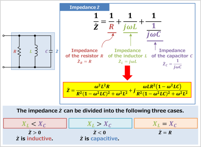
The impedance \({\dot{Z}}_R\) of the resistor \(R\), the impedance \({\dot{Z}}_L\) of the inductor \(L\), and the impedance \({\dot{Z}}_C\) of the capacitor \(C\) can be expressed by the following equations:
\begin{eqnarray}
{\dot{Z}_R}&=&R\tag{1}\\
\\
{\dot{Z}_L}&=&jX_L=j{\omega}L\tag{2}\\
\\
{\dot{Z}_C}&=&-jX_C=-j\frac{1}{{\omega}C}=\frac{1}{j{\omega}C}\tag{3}
\end{eqnarray}
, where \({\omega}\) is the angular frequency, which is equal to \(2{\pi}f\), and \(X_L\left(={\omega}L\right)\) is called inductive reactance, which is the resistive component of inductor \(L\) and \(X_C\left(=\displaystyle\frac{1}{{\omega}C}\right)\) is called capacitive reactance, which is the resistive component of capacitor \(C\).
The sum of the reciprocals of each impedance is the reciprocal of the impedance \({\dot{Z}}\) of the RLC parallel circuit. Therefore, it can be expressed by the following equation:
\begin{eqnarray}
\frac{1}{{\dot{Z}}}&=&\frac{1}{{\dot{Z}_R}}+\frac{1}{{\dot{Z}_L}}+\frac{1}{{\dot{Z}_C}}\\
\\
&=&\frac{1}{R}+\frac{1}{j{\omega}L}+\frac{1}{\displaystyle\frac{1}{j{\omega}C}}\\
\\
&=&\frac{1}{R}+\frac{1}{j{\omega}L}+j{\omega}C\\
\\
&=&\frac{j{\omega}L+R+j{\omega}C×j{\omega}LR}{j{\omega}LR}\\
\\
&=&\frac{j{\omega}L+R+j^2{\omega}^2LCR}{j{\omega}LR}\\
\\
&=&\frac{j{\omega}L+R-{\omega}^2LCR}{j{\omega}LR}\\
\\
&=&\frac{R(1-{\omega}^2LC)+j{\omega}L}{j{\omega}LR}\tag{4}
\end{eqnarray}
From equation (4), by interchanging the denominator and numerator, the following equation is obtained:
\begin{eqnarray}
{\dot{Z}}=\frac{1}{\displaystyle\frac{1}{R}+\displaystyle\frac{1}{j{\omega}L}+j{\omega}C}=\frac{j{\omega}LR}{R(1-{\omega}^2LC)+j{\omega}L}\tag{5}
\end{eqnarray}
From equation (5), there is an imaginary unit \(j\) in the denominator. To make sure that only the numerator has an imaginary unit \(j\), multiply the denominator and numerator by "\(\{R(1-{\omega}^2LC)-j{\omega}L\}\)".
\begin{eqnarray}
{\dot{Z}}&=&\frac{j{\omega}LR\{R(1-{\omega}^2LC)-j{\omega}L\}}{\{R(1-{\omega}^2LC)+j{\omega}L\}\{R(1-{\omega}^2LC)-j{\omega}L\}}\\
\\
&=&\frac{j{\omega}LR^2(1-{\omega}^2LC)-j^2{\omega}^2L^2R}{R^2(1-{\omega}^2LC)^2-j{\omega}LR(1-{\omega}^2LC)+j{\omega}LR(1-{\omega}^2LC)-j^2{\omega}^2L^2}\\
\\
&=&\frac{j{\omega}LR^2(1-{\omega}^2LC)+{\omega}^2L^2R}{R^2(1-{\omega}^2LC)^2-j{\omega}LR(1-{\omega}^2LC)+j{\omega}LR(1-{\omega}^2LC)+{\omega}^2L^2}\\
\\
&=&\frac{{\omega}^2L^2R+j{\omega}LR^2(1-{\omega}^2LC)}{R^2(1-{\omega}^2LC)^2+{\omega}^2L^2}\\
\\
&=&\frac{{\omega}^2L^2R}{R^2(1-{\omega}^2LC)^2+{\omega}^2L^2}+j\frac{{\omega}LR^2(1-{\omega}^2LC)}{R^2(1-{\omega}^2LC)^2+{\omega}^2L^2}\tag{6}
\end{eqnarray}
From the above, the impedance \({\dot{Z}}\) of the RLC parallel circuit can be expressed as:
The impedance of the RLC parallel circuit
\begin{eqnarray}
{\dot{Z}}&=&\frac{1}{\displaystyle\frac{1}{R}+\displaystyle\frac{1}{j{\omega}L}+j{\omega}C}\\
\\
&=&\frac{{\omega}^2L^2R}{R^2(1-{\omega}^2LC)^2+{\omega}^2L^2}+j\frac{{\omega}LR^2(1-{\omega}^2LC)}{R^2(1-{\omega}^2LC)^2+{\omega}^2L^2}\tag{7}
\end{eqnarray}
The magnitude of the inductive reactance \(X_L(={\omega}L)\) and capacitive reactance \(X_C\left(=\displaystyle\frac{1}{{\omega}C}\right)\) determine whether the impedance \({\dot{Z}}\) of the RLC parallel circuit is inductive or capacitive.
- In the case of \(X_L{\;}{\lt}{\;}X_C\)
- In the case of \(X_L{\;}{\gt}{\;}X_C\)
- In the case of \(X_L=X_C\)
In the case of \(X_L{\;}{\lt}{\;}X_C\)
If the inductive reactance \(X_L\) is smaller than the capacitive reactance \(X_C\), the following equation holds.
\begin{eqnarray}
&&X_L{\;}{\lt}{\;}X_C\\
\\
{\Leftrightarrow}&&{\omega}L{\;}{\lt}{\;}\displaystyle\frac{1}{{\omega}C}\\
\\
{\Leftrightarrow}&&{\omega}^2LC{\;}{\lt}{\;}1\\
\\
{\Leftrightarrow}&&1-{\omega}^2LC{\;}{\gt}{\;}0\tag{8}
\end{eqnarray}
In this case, the imaginary part \(\displaystyle\frac{{\omega}LR^2(1-{\omega}^2LC)}{R^2(1-{\omega}^2LC)^2+{\omega}^2L^2}\) of the impedance \({\dot{Z}}\) of the RLC parallel circuit becomes "positive" (in other words, the value multiplied by the imaginary unit "\(j\)" becomes "positive"), so the impedance \({\dot{Z}}\) is inductive.
In the case of \(X_L{\;}{\gt}{\;}X_C\)
If the inductive reactance \(X_L\) is bigger than the capacitive reactance \(X_C\), the following equation holds.
\begin{eqnarray}
&&X_L{\;}{\gt}{\;}X_C\\
\\
{\Leftrightarrow}&&{\omega}L{\;}{\gt}{\;}\displaystyle\frac{1}{{\omega}C}\\
\\
{\Leftrightarrow}&&{\omega}^2LC{\;}{\gt}{\;}1\\
\\
{\Leftrightarrow}&&1-{\omega}^2LC{\;}{\lt}{\;}0\tag{9}
\end{eqnarray}
In this case, the imaginary part \(\displaystyle\frac{{\omega}LR^2(1-{\omega}^2LC)}{R^2(1-{\omega}^2LC)^2+{\omega}^2L^2}\) of the impedance \({\dot{Z}}\) of the RLC parallel circuit becomes "negative" (in other words, the value multiplied by the imaginary unit "\(j\)" becomes "negative"), so the impedance \({\dot{Z}}\) is capacitive.
In the case of \(X_L=X_C\)
If the inductive reactance is equal to the capacitive reactance, the following equation holds.
\begin{eqnarray}
&&X_L=X_C\\
\\
{\Leftrightarrow}&&{\omega}L=\displaystyle\frac{1}{{\omega}C}\\
\\
{\Leftrightarrow}&&{\omega}^2LC=1\\
\\
{\Leftrightarrow}&&1-{\omega}^2LC=0\tag{10}
\end{eqnarray}
In this case, the impedance \({\dot{Z}}\) of the RLC parallel circuit is given by:
\begin{eqnarray}
{\dot{Z}}&=&\frac{{\omega}^2L^2R}{R^2(1-{\omega}^2LC)^2+{\omega}^2L^2}+j\frac{{\omega}LR^2(1-{\omega}^2LC)}{R^2(1-{\omega}^2LC)^2+{\omega}^2L^2}\\
\\
&=&\frac{{\omega}^2L^2R}{R^2×0^2+{\omega}^2L^2}+j\frac{{\omega}LR^2×0}{R^2×0^2+{\omega}^2L^2}\\
\\
&=&R\tag{11}
\end{eqnarray}
In this case, the circuit is in parallel resonance. When parallel resonance is established, the part of the parallel circuit between the inductor \(L\) and the capacitor \(C\) is open. Therefore, the impedance \({\dot{Z}}\) of the RLC parallel circuit is "\({\dot{Z}}=R\)". In this case, the angular frequency \({\omega}\) and frequency \(f\) are as follows:
\begin{eqnarray}
X_L&=&X_C\\
\\
{\omega}L&=&\frac{1}{{\omega}C}\\
\\
{\Leftrightarrow}{\omega}&=&\frac{1}{\displaystyle\sqrt{LC}}\\
\\
{\Leftrightarrow}f&=&\frac{1}{2{\pi}\displaystyle\sqrt{LC}}\tag{12}
\end{eqnarray}
Magnitude of the impedance of the RLC parallel circuit
We have just obtained the impedance \({\dot{Z}}\) expressed by the following equation.
\begin{eqnarray}
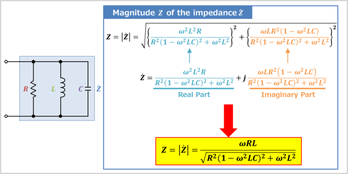
{\dot{Z}}=\frac{{\omega}^2L^2R}{R^2(1-{\omega}^2LC)^2+{\omega}^2L^2}+j\frac{{\omega}LR^2(1-{\omega}^2LC)}{R^2(1-{\omega}^2LC)^2+{\omega}^2L^2}\tag{13}
\end{eqnarray}
The magnitude \(Z\) of the impedance of the RLC parallel circuit is the absolute value of the impedance \({\dot{Z}}\) in equation (13).
In more detail, the magnitude \(Z\) of the impedance \({\dot{Z}}\) can be obtained by adding the square of the real part \(\displaystyle\frac{{\omega}^2L^2R}{R^2(1-{\omega}^2LC)^2+{\omega}^2L^2}\) and the square of the imaginary part \(\displaystyle\frac{{\omega}LR^2(1-{\omega}^2LC)}{R^2(1-{\omega}^2LC)^2+{\omega}^2L^2}\) and taking the square root, which can be expressed in the following equation:
\begin{eqnarray}
Z&=&|{\dot{Z}}|\\
\\
&=&\displaystyle\sqrt{\left\{\frac{{\omega}^2L^2R}{R^2(1-{\omega}^2LC)^2+{\omega}^2L^2}\right\}^2+\left\{\frac{{\omega}LR^2(1-{\omega}^2LC)}{R^2(1-{\omega}^2LC)^2+{\omega}^2L^2}\right\}^2}\\
\\
&=&\displaystyle\sqrt{\frac{{\omega}^4L^4R^2+{\omega}^2L^2R^4(1-{\omega}^2LC)^2}{\left\{R^2(1-{\omega}^2LC)^2+{\omega}^2L^2\right\}^2}}\\
\\
&=&\displaystyle\sqrt{\frac{{\omega}^2L^2R^2\left\{{\omega}^2L^2+R^2(1-{\omega}^2LC)^2\right\}}{\left\{R^2(1-{\omega}^2LC)^2+{\omega}^2L^2\right\}^2}}\\
\\
&=&\displaystyle\sqrt{\frac{{\omega}^2L^2R^2\left\{R^2(1-{\omega}^2LC)^2+{\omega}^2L^2\right\}}{\left\{R^2(1-{\omega}^2LC)^2+{\omega}^2L^2\right\}^2}}\\
\\
&=&\displaystyle\sqrt{\frac{{\omega}^2L^2R^2}{R^2(1-{\omega}^2LC)^2+{\omega}^2L^2}}\\
\\
&=&\frac{{\omega}LR}{\sqrt{R^2(1-{\omega}^2LC)^2+{\omega}^2L^2}}\tag{14}
\end{eqnarray}
Next, to express equation (14) in terms of "inductive reactance \(X_L\)" and "capacitive reactance \(X_C\)", the denominator and numerator are divided by \({\omega}L\).
\begin{eqnarray}
Z&=&\frac{\displaystyle\frac{{\omega}LR}{{\omega}LR}}{\sqrt{\displaystyle\frac{1}{{\omega}^2L^2R^2}\left\{R^2(1-{\omega}^2LC)^2+{\omega}^2L^2\right\}}}\\
\\
&=&\frac{1}{\sqrt{\displaystyle\frac{1}{{\omega}^2L^2}(1-{\omega}^2LC)^2+\displaystyle\frac{1}{R^2}}}\\
\\
&=&\frac{1}{\sqrt{\left(\displaystyle\frac{1}{R}\right)^2+\left(\displaystyle\frac{1}{{\omega}L}-{\omega}C\right)^2}}\\
\\
&=&\frac{1}{\sqrt{\left(\displaystyle\frac{1}{R}\right)^2+\left(\displaystyle\frac{1}{X_L}-\displaystyle\frac{1}{X_C}\right)^2}}\tag{15}
\end{eqnarray}
From the above, the magnitude \(Z\) of the impedance of the RLC parallel circuit can be expressed as:
The magnitude of the impedance of the RLC parallel circuit
\begin{eqnarray}
Z&=&|{\dot{Z}}|\\
\\
&=&\frac{{\omega}LR}{\sqrt{R^2(1-{\omega}^2LC)^2+{\omega}^2L^2}}\\
\\
&=&\frac{1}{\sqrt{\left(\displaystyle\frac{1}{R}\right)^2+\left(\displaystyle\frac{1}{{\omega}L}-{\omega}C\right)^2}}\\
\\
&=&\frac{1}{\sqrt{\left(\displaystyle\frac{1}{R}\right)^2+\left(\displaystyle\frac{1}{X_L}-\displaystyle\frac{1}{X_C}\right)^2}}\tag{16}
\end{eqnarray}
Supplement
Some impedance \(Z\) symbols have a ". (dot)" above them and are labeled \({\dot{Z}}\).
\({\dot{Z}}\) with this dot represents a vector.
If it has a dot (e.g. \({\dot{Z}}\)), it represents a vector (complex number), and if it does not have a dot (e.g. \(Z\)), it represents the absolute value (magnitude, length) of the vector.
Vector diagram of the RLC parallel circuit
The vector diagram of the impedance \({\dot{Z}}\) of the RLC parallel circuit can be drawn in the following steps.
How to draw a Vector Diagram
- Draw the vector of impedance \({\dot{Z}_{RE}}\) of the real part of impedance \({\dot{Z}}\)
- Draw the vector of impedance \({\dot{Z}_{IM}}\) of the imaginary part of impedance \({\dot{Z}}\)
- Combine the vectors
Let's take a look at each step in turn.
Draw the vector of impedance \({\dot{Z}_{RE}}\) of the real part of impedance \({\dot{Z}}\)
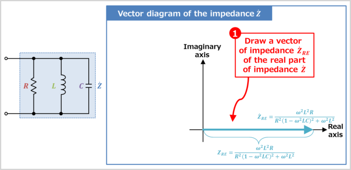
The impedance \({\dot{Z}_{RE}}\) of the real part of impedance \({\dot{Z}}\) is expressed by:
\begin{eqnarray}
{\dot{Z}_{RE}}=\frac{{\omega}^2L^2R}{R^2(1-{\omega}^2LC)^2+{\omega}^2L^2}\tag{17}
\end{eqnarray}
Therefore, the vector direction of the impedance \({\dot{Z}_{RE}}\) is the direction of the real axis. How to determine the vector orientation will be explained in more detail later.
The magnitude (length) \(Z_{RE}\) of the vector of impedances \({\dot{Z}_{RE}}\) of the real part is given by
\begin{eqnarray}
Z_{RE}=|{\dot{Z}_{RE}}|=\displaystyle\sqrt{\left(\frac{{\omega}^2L^2R}{R^2(1-{\omega}^2LC)^2+{\omega}^2L^2}\right)^2}=\frac{{\omega}^2L^2R}{R^2(1-{\omega}^2LC)^2+{\omega}^2L^2}\tag{18}
\end{eqnarray}
Draw the vector of impedance \({\dot{Z}_{IM}}\) of the imaginary part of impedance \({\dot{Z}}\)
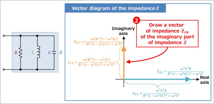
The impedance \({\dot{Z}_{IM}}\) of the imaginary part of impedance \({\dot{Z}}\) is expressed by:
\begin{eqnarray}
{\dot{Z}_{IM}}=j\frac{{\omega}LR^2(1-{\omega}^2LC)}{R^2(1-{\omega}^2LC)^2+{\omega}^2L^2}\tag{19}
\end{eqnarray}
The vector direction of the impedance \({\dot{Z}_{IM}}\) depends on the magnitude of the "inductive reactance \(X_L\)" and "capacitive reactance \(X_C\)" shown below.
- In the case of \(X_L{\;}{\lt}{\;}X_C\)
- In the case of \(X_L{\;}{\gt}{\;}X_C\)
- In the case of \(X_L=X_C\)
We will now discuss the vector direction of the impedance \({\dot{Z}_{IM}}\) in case "\(X_L{\;}{\lt}{\;}X_C\)"(we will discuss the vector direction in each case later).
If the inductive reactance \(X_L\) is smaller than the capacitive reactance \(X_C\), then "\(1-{\omega}^2LC{\;}{\gt}{\;}0\)".
Therefore, since the value \(\displaystyle\frac{{\omega}LR^2(1-{\omega}^2LC)}{R^2(1-{\omega}^2LC)^2+{\omega}^2L^2}\) multiplied by the imaginary unit "\(j\)" of the impedance \({\dot{Z}_{IM}}\) is positive, the vector direction of the impedance \({\dot{Z}_{IM}}\) is 90° counterclockwise around the real axis. How to determine the vector orientation will be explained in more detail later.
The magnitude (length) \(Z_{IM}\) of the vector of impedances \({\dot{Z}_{IM}}\) of the imaginary part is given by
\begin{eqnarray}
Z_{IM}=|{\dot{Z}_{IM}}|=\displaystyle\sqrt{\left(\frac{{\omega}LR^2(1-{\omega}^2LC)}{R^2(1-{\omega}^2LC)^2+{\omega}^2L^2}\right)^2}=\frac{{\omega}LR^2(1-{\omega}^2LC)}{R^2(1-{\omega}^2LC)^2+{\omega}^2L^2}\tag{20}
\end{eqnarray}
Combine the vectors

Combining the vector of "impedance \({\dot{Z}}_{RE}\) of the real part" and "impedance \({\dot{Z}}_{IM}\) of the imaginary part" is the vector diagram of the impedance \({\dot{Z}}\) of the RLC parallel circuit.
Again, the impedance \({\dot{Z}}\) of an RLC parallel circuit is expressed by:
\begin{eqnarray}
{\dot{Z}}&=&\frac{{\omega}^2L^2R}{R^2(1-{\omega}^2LC)^2+{\omega}^2L^2}+j\frac{{\omega}LR^2(1-{\omega}^2LC)}{R^2(1-{\omega}^2LC)^2+{\omega}^2L^2}\tag{21}
\end{eqnarray}
The vector direction of the impedance \({\dot{Z}}\) of an RLC parallel circuit depends on the magnitude of the "inductive reactance \(X_L\)" and "capacitive reactance \(X_C\)" shown below.
- In the case of \(X_L{\;}{\lt}{\;}X_C\)
- In the case of \(X_L{\;}{\gt}{\;}X_C\)
- In the case of \(X_L=X_C\)
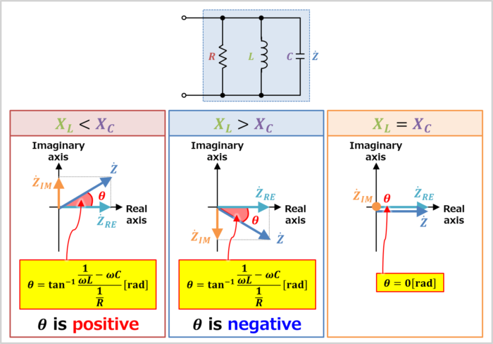
In the case of \(X_L{\;}{\lt}{\;}X_C\)
If the inductive reactance \(X_L\) is smaller than the capacitive reactance \(X_C\), then "\(1-{\omega}^2LC{\;}{\gt}{\;}0\)".
Therefore, since the value \(\displaystyle\frac{{\omega}LR^2(1-{\omega}^2LC)}{R^2(1-{\omega}^2LC)^2+{\omega}^2L^2}\) multiplied by the imaginary unit "\(j\)" of the impedance \({\dot{Z}_{IM}}\) is positive, the vector direction of the impedance \({\dot{Z}_{IM}}\) is 90° counterclockwise around the real axis. How to determine the vector orientation will be explained in more detail later.
Hence, the vector direction of the impedance \({\dot{Z}}\) is upward to the right.
In the case of \(X_L{\;}{\gt}{\;}X_C\)
If the inductive reactance \(X_L\) is bigger than the capacitive reactance \(X_C\), then "\(1-{\omega}^2LC{\;}{\lt}{\;}0\)".
Therefore, since the value \(\displaystyle\frac{{\omega}LR^2(1-{\omega}^2LC)}{R^2(1-{\omega}^2LC)^2+{\omega}^2L^2}\) multiplied by the imaginary unit "\(j\)" of the impedance \({\dot{Z}_{IM}}\) is negative, the vector direction of the impedance \({\dot{Z}_{IM}}\) is 90° clockwise around the real axis. How to determine the vector orientation will be explained in more detail later.
Hence, the vector direction of the impedance \({\dot{Z}}\) is downward to the right.
In the case of \(X_L=X_C\)
If the inductive reactance is equal to the capacitive reactance, then "\(1-{\omega}^2LC=0\)".
In this case, the vector direction of the impedance \({\dot{Z}}\) is to the right because the impedance \({\dot{Z}}\) of the RLC parallel circuit is "\({\dot{Z}}=R\)".
Vector orientation
Here is a more detailed explanation of how vector orientation is determined.
Vector orientation
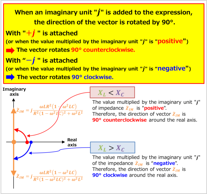
When an imaginary unit "\(j\)" is added to the expression, the direction of the vector is rotated by 90°.
- With "\(+j\)" is attached(or when the value multiplied by the imaginary unit "\(j\)" is "positive")
- The vector rotates 90° counterclockwise.
- With "\(-j\)" is attached(or when the value multiplied by the imaginary unit "\(j\)" is "negative")
- The vector rotates 90° clockwise.
The impedance \({\dot{Z}}\) of an RLC parallel circuit is expressed by the following equation:
\begin{eqnarray}
{\dot{Z}_{IM}}=j\frac{{\omega}LR^2(1-{\omega}^2LC)}{R^2(1-{\omega}^2LC)^2+{\omega}^2L^2}\tag{22}
\end{eqnarray}
In the case of \(X_L{\;}{\lt}{\;}X_C\), since "\(1-{\omega}^2LC{\;}{\gt}{\;}0\)", the value multiplied by the imaginary unit "\(j\)" of the impedance \({\dot{Z}_{IM}}\) is "positive". Therefore, the direction of vector \({\dot{Z}_{IM}}\) is 90° counterclockwise around the real axis.
In the case of \(X_L{\;}{\gt}{\;}X_C\), since "\(1-{\omega}^2LC{\;}{\lt}{\;}0\)", the value multiplied by the imaginary unit "\(j\)" of the impedance \({\dot{Z}_{IM}}\) is "negative". Therefore, the direction of vector \({\dot{Z}_{IM}}\) is 90° clockwise around the real axis.
Impedance phase angle of the RLC parallel circuit
The impedance phase angle \({\theta}\) of the RLC parallel circuit can be obtained from the vector diagram.
\begin{eqnarray}
{\tan}{\theta}&=&\displaystyle\frac{\displaystyle\frac{{\omega}LR^2(1-{\omega}^2LC)}{R^2(1-{\omega}^2LC)^2+{\omega}^2L^2}}{\displaystyle\frac{{\omega}^2L^2R}{R^2(1-{\omega}^2LC)^2+{\omega}^2L^2}}\\
\\
&=&\displaystyle\frac{{\omega}LR^2(1-{\omega}^2LC)}{{\omega}^2L^2R}\tag{23}
\end{eqnarray}
Next, to express equation (23) in terms of "inductive reactance \(X_L\)" and "capacitive reactance \(X_C\)", the denominator and numerator are divided by \({\omega}^2L^2R^2\).
\begin{eqnarray}
{\tan}{\theta}&=&\displaystyle\frac{\displaystyle\frac{{\omega}LR^2(1-{\omega}^2LC)}{{\omega}^2L^2R^2}}{\displaystyle\frac{{\omega}^2L^2R}{{\omega}^2L^2R^2}}\\
\\
&=&\displaystyle\frac{\displaystyle\frac{1}{{\omega}L}-{\omega}C}{\displaystyle\frac{1}{R}}\\
\\
&=&\displaystyle\frac{\displaystyle\frac{1}{X_L}-\displaystyle\frac{1}{X_C}}{\displaystyle\frac{1}{R}}\tag{24}
\end{eqnarray}
From the above, the impedance phase angle \({\theta}\) of the RLC parallel circuit is expressed by the following equation:
Impedance phase angle of the RLC parallel circuit
\begin{eqnarray}
{\theta}&=&{\tan}^{-1}\displaystyle\frac{\displaystyle\frac{1}{{\omega}L}-{\omega}C}{\displaystyle\frac{1}{R}}{\mathrm{[rad]}}\\
\\
&=&{\tan}^{-1}\displaystyle\frac{\displaystyle\frac{1}{X_L}-\displaystyle\frac{1}{X_C}}{\displaystyle\frac{1}{R}}{\mathrm{[rad]}}\tag{25}
\end{eqnarray}
The magnitude of the inductive reactance \(X_L(={\omega}L)\) and capacitive reactance \(X_C\left(=\displaystyle\frac{1}{{\omega}C}\right)\) determine whether the impedance phase angle \({\theta}\) of the RLC parallel circuit is positive or negative.
- In the case of \(X_L{\;}{\lt}{\;}X_C\)
- In the case of \(X_L{\;}{\gt}{\;}X_C\)
- In the case of \(X_L=X_C\)
In the case of \(X_L{\;}{\lt}{\;}X_C\)
If the inductive reactance \(X_L\) is smaller than the capacitive reactance \(X_C\), the following equation holds.
\begin{eqnarray}
&&X_L{\;}{\lt}{\;}X_C\\
\\
{\Leftrightarrow}&&\frac{1}{X_L}-\frac{1}{X_C}{\;}{\gt}{\;}0\tag{26}
\end{eqnarray}
Therefore, the impedance phase angle \({\theta}\) of the RLC parallel circuit is "positive".
In the case of \(X_L{\;}{\gt}{\;}X_C\)
If the inductive reactance \(X_L\) is bigger than the capacitive reactance \(X_C\), the following equation holds.
\begin{eqnarray}
&&X_L{\;}{\gt}{\;}X_C\\
\\
{\Leftrightarrow}&&\frac{1}{X_L}-\frac{1}{X_C}{\;}{\lt}{\;}0\tag{27}
\end{eqnarray}
Therefore, the impedance phase angle \({\theta}\) of the RLC parallel circuit is "negative".
In the case of \(X_L=X_C\)
If the inductive reactance is equal to the capacitive reactance, the following equation holds.
\begin{eqnarray}
&&X_L=X_C\\
\\
{\Leftrightarrow}&&\frac{1}{X_L}-\frac{1}{X_C}=0\tag{28}
\end{eqnarray}
Therefore, the impedance phase angle \({\theta}\) of the RLC parallel circuit is "\({\theta}=0{\mathrm{[rad]}}\)".
Summary
In this article, the following information on "RLC parallel circuit was explained.
- Equation, magnitude, vector diagram, and impedance phase angle of RLC parallel circuit impedance
Thank you for reading.
Related article
Related articles on impedance in series and parallel circuits are listed below. If you are interested, please check the link below.
- RL Series Circuit (Impedance, Phasor Diagram)
- RC Series Circuit (Impedance, Phasor Diagram)
- LC Series Circuit (Impedance, Phasor Diagram)
- RLC Series Circuit (Impedance, Phasor Diagram)
- RL Parallel Circuit (Impedance, Phasor Diagram)
- RC Parallel Circuit (Impedance, Phasor Diagram)
- LC Parallel Circuit (Impedance, Phasor Diagram)