RLC Parallel Circuit (Admittance, Phasor Diagram)

Regarding the RLC parallel circuit, this article will explain the information below.

• Equation, magnitude, vector diagram, and admittance phase angle of RLC parallel circuit admittance

Admittance of the RLC parallel circuit

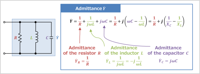
An RLC parallel circuit is an electrical circuit consisting of a resistor \(R\), an inductor \(L\), and a capacitor \(C\) connected in parallel, driven by a voltage source or current source.

The impedance \({\dot{Z}}_R\) of the resistor \(R\), the impedance \({\dot{Z}}_L\) of the inductor \(L\), and the impedance \({\dot{Z}}_C\) of the capacitor \(C\) can be expressed by the following equations:

\begin{eqnarray}
{\dot{Z}_R}&=&R\tag{1}\\
\\
{\dot{Z}_L}&=&jX_L=j{\omega}L\tag{2}\\
\\
{\dot{Z}_C}&=&-jX_C=-j\frac{1}{{\omega}C}=\frac{1}{j{\omega}C}\tag{3}
\end{eqnarray}

, where \({\omega}\) is the angular frequency, which is equal to \(2{\pi}f\), and \(X_L\left(={\omega}L\right)\) is called inductive reactance, which is the resistive component of inductor \(L\) and \(X_C\left(=\displaystyle\frac{1}{{\omega}C}\right)\) is called capacitive reactance, which is the resistive component of capacitor \(C\).

Since admittance is the reciprocal of impedance, the admittance \({\dot{Y}}_R\) of resistor \(R\), the admittance \({\dot{Y}}_L\) of inductor \(L\), and the admittance \({\dot{Y}}_C\) of capacitor \(C\) can each be expressed by the following equations.

\begin{eqnarray}
{\dot{Y}_R}&=&\frac{1}{{\dot{Z}_R}}=\frac{1}{R}\tag{4}\\
\\
{\dot{Y}_L}&=&\frac{1}{{\dot{Z}_L}}=\frac{1}{j{\omega}L}=-j\frac{1}{{\omega}L}\tag{5}\\
\\
{\dot{Y}_C}&=&\frac{1}{{\dot{Z}_C}}=\frac{1}{\displaystyle\frac{1}{j{\omega}C}}=j{\omega}C\tag{6}
\end{eqnarray}

The admittance \({\dot{Y}}\) of the RLC parallel circuit is the sum of the respective admittances, and is as follows:

\begin{eqnarray}
{\dot{Y}}&=&{\dot{Y}_R}+{\dot{Y}_L}+{\dot{Y}_C}\\
\\
&=&\frac{1}{R}+\frac{1}{j{\omega}L}+j{\omega}C\\
\\
&=&\frac{1}{R}-j\frac{1}{{\omega}L}+j{\omega}C\\
\\
&=&\frac{1}{R}+j\left({\omega}C-\frac{1}{{\omega}L}\right)\\
\\
&=&\frac{1}{R}+j\left(\frac{1}{X_C}-\frac{1}{X_L}\right)\tag{7}
\end{eqnarray}

From the above, the admittance \({\dot{Y}}\) of the RLC parallel circuit becomes the following equation.

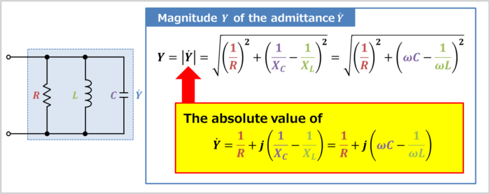
Magnitude of the admittance of the RLC parallel circuit

We have just obtained the admittance \({\dot{Y}}\) expressed by the following equation.

\begin{eqnarray}
{\dot{Y}}&=&\frac{1}{R}+j\left({\omega}C-\frac{1}{{\omega}L}\right){\mathrm{[S]}}\\
\\
&=&\frac{1}{R}+j\left(\frac{1}{X_C}-\frac{1}{X_L}\right){\mathrm{[S]}}\tag{9}
\end{eqnarray}

The magnitude \(Y\) of the admittance of the RLC parallel circuit is the absolute value of the admittance \({\dot{Y}}\) in equation (9).

In more detail, the magnitude \(Y\) of the admittance \({\dot{Y}}\) can be obtained by adding the square of the real part \(\left(\displaystyle\frac{1}{R}\right)\) and the square of the imaginary part \(\left(\displaystyle\frac{1}{X_C}-\displaystyle\frac{1}{X_L}\right)\) and taking the square root, which can be expressed in the following equation.

\begin{eqnarray}
Y&=&|{\dot{Y}}|\\
\\
&=&\sqrt{\left(\frac{1}{R}\right)^2+\left(\frac{1}{X_C}-\frac{1}{X_L}\right)^2}\\
\\
&=&\sqrt{\left(\frac{1}{R}\right)^2+\left({\omega}C-\frac{1}{{\omega}L}\right)^2}\\
\\
&=&\sqrt{\frac{\left(\displaystyle\frac{1}{R}\right)^2×{\omega}^2L^2R^2+\left({\omega}C-\displaystyle\frac{1}{{\omega}L}\right)^2×{\omega}^2L^2R^2}{{\omega}^2L^2R^2}}\\
\\
&=&\sqrt{\frac{{\omega}^2L^2+\left({\omega}^2LC-1\right)^2×R^2}{{\omega}^2L^2R^2}}\\
\\
&=&\frac{\sqrt{{\omega}^2L^2+R^2\left({\omega}^2LC-1\right)^2}}{{\omega}LR}\tag{10}
\end{eqnarray}

From the above, the magnitude \(Y\) of the admittance \({\dot{Y}}\) of the RLC parallel circuit becomes the following equation.

Vector diagram of the RLC parallel circuit

The vector diagram of the admittance \({\dot{Y}}\) of the RLC parallel circuit can be drawn in the following steps.

Let's take a look at each step in turn.

Draw a vector of admittance \({\dot{Y}}_R\) of resistor \(R\)

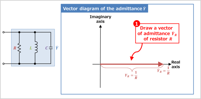
The admittance \({\dot{Y}}_R\) of resistor \(R\) is expressed by the following equation.

\begin{eqnarray}
{\dot{Y}_R}=\frac{1}{R}\tag{12}
\end{eqnarray}

Therefore, the vector direction of the admittance \({\dot{Y}}_R\) is the direction of the real axis. If the expression does not have an imaginary unit \(j\), the vector does not rotate and is oriented on the real axis. How to determine the vector orientation will be explained in more detail later.

Also, the magnitude (length) \(Y_R\) of the vector of the admittance \({\dot{Y}}_R\) is expressed by the following equation.

\begin{eqnarray}
Y_R=|{\dot{Y}_R}|=\displaystyle\sqrt{\left(\frac{1}{R}\right)^2}=\frac{1}{R}\tag{13}
\end{eqnarray}

Draw a vector of admittance \({\dot{Y}}_L\) of inductor \(L\)

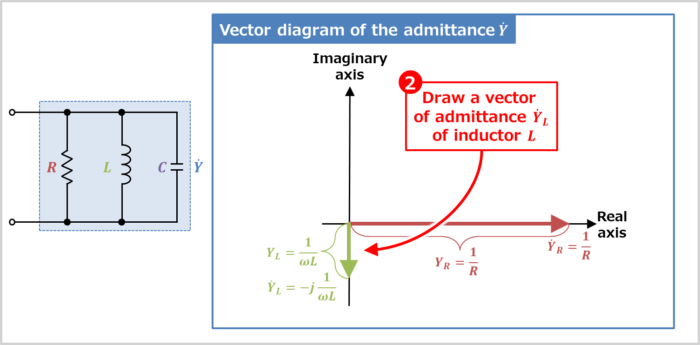
The admittance \({\dot{Y}}_L\) of inductor \(L\) is expressed by the following equation.

\begin{eqnarray}
{\dot{Y}_L}=-j\frac{1}{{\omega}L}\tag{14}
\end{eqnarray}

Therefore, the orientation of the admittance \({\dot{Y}}_L\) vector is 90° counterclockwise around the real axis. When "\(-j\)" is added to the equation, the vector is rotated 90° clockwise. How to determine the vector orientation will be explained in detail later.

Also, the magnitude (length) \(Y_L\) of the vector of the admittance \({\dot{Y}}_L\) is expressed by the following equation.

\begin{eqnarray}
Y_L=|{\dot{Y}_L}|=\displaystyle\sqrt{\left(\frac{1}{{\omega}L}\right)^2}=\frac{1}{{\omega}L}=\frac{1}{X_L}\tag{15}
\end{eqnarray}

Draw a vector of admittance \({\dot{Y}}_C\) of capacitor \(C\)

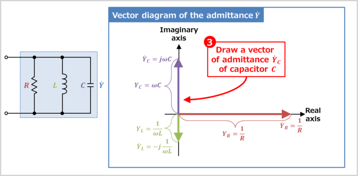
The admittance \({\dot{Y}}_C\) of capacitor \(C\) is expressed by the following equation.

\begin{eqnarray}
{\dot{Y}_C}=j{\omega}C\tag{16}
\end{eqnarray}

Therefore, the orientation of the admittance \({\dot{Y}}_C\) vector is 90° counterclockwise around the real axis. When "\(+j\)" is added to the equation, the vector is rotated 90° counterclockwise. How to determine the vector orientation will be explained in detail later.

Also, the magnitude (length) \(Y_C\) of the vector of the admittance \({\dot{Y}}_C\) is expressed by the following equation.

\begin{eqnarray}
Y_C=|{\dot{Y}_C}|=\displaystyle\sqrt{\left({\omega}C\right)^2}={\omega}C=\frac{1}{X_C}\tag{17}
\end{eqnarray}

Combine the vectors

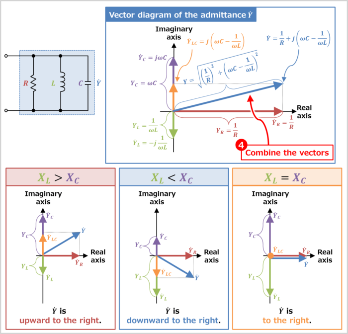
Combining the vector of "admittance \({\dot{Y}}_R\) of resistor \(R\)", "admittance \({\dot{Y}}_L\) of inductor \(L\)", and "admittance \({\dot{Y}}_C\) of capacitor \(C\)" is the vector diagram of the admittance \({\dot{Y}}\) of the RLC parallel circuit.

We have just explained that the admittance \({\dot{Y}}\) of an RLC parallel circuit and its magnitude \(Y\) are expressed by the following equation

\begin{eqnarray}
{\dot{Y}}&=&\frac{1}{R}+j\left({\omega}C-\frac{1}{{\omega}L}\right){\mathrm{[S]}}\tag{18}\\
\\
Y&=&\sqrt{\left(\frac{1}{R}\right)^2+\left({\omega}C-\frac{1}{{\omega}L}\right)^2}{\mathrm{[S]}}\tag{19}
\end{eqnarray}

In the above equation, the vector direction of admittance \({\dot{Y}}\) of the RLC parallel circuit changes depending on the magnitude of "inductive reactance \(X_L={\omega}L\)" and "capacitive reactance \(X_C=\displaystyle\frac{1}{{\omega}C}\)".

• In Case \(X_L{\;}{\gt}{\;}X_C\)
• In Case \(X_L{\;}{\lt}{\;}X_C\)
• In Case \(X_L=X_C\)

In Case \(X_L{\;}{\gt}{\;}X_C\)

If "inductive reactance \(X_L\)" is larger than "capacitive reactance \(X_C\)", the following equation holds.

\begin{eqnarray}
&&X_L{\;}{\gt}{\;}X_C\\
\\
{\Leftrightarrow}&&\frac{1}{Y_L}{\;}{\gt}{\;}\frac{1}{Y_C}\\
\\
{\Leftrightarrow}&&Y_L{\;}{\lt}{\;}Y_C\tag{20}
\end{eqnarray}

The vector direction of admittance \({\dot{Y}}\) of the RLC parallel circuit is upward to the right, because "the magnitude \(Y_L\) of admittance of inductor \(L\)" is smaller than "the magnitude \(Y_C\) of admittance of capacitor \(C\)".

In Case \(X_L{\;}{\lt}{\;}X_C\)

If "inductive reactance \(X_L\)" is smaller than "capacitive reactance \(X_C\)", the following equation holds.

\begin{eqnarray}
&&X_L{\;}{\lt}{\;}X_C\\
\\
{\Leftrightarrow}&&\frac{1}{Y_L}{\;}{\lt}{\;}\frac{1}{Y_C}\\
\\
{\Leftrightarrow}&&Y_L{\;}{\gt}{\;}Y_C\tag{21}
\end{eqnarray}

The vector direction of admittance \({\dot{Y}}\) of the RLC parallel circuit is downward to the right, because "the magnitude \(Y_L\) of admittance of inductor \(L\)" is larger than "the magnitude \(Y_C\) of admittance of capacitor \(C\)".

In Case \(X_L=X_C\)

If "inductive reactance \(X_L\)" is equal to "capacitive reactance \(X_C\)", the following equation holds.

\begin{eqnarray}
&&X_L=X_C\\
\\
{\Leftrightarrow}&&\frac{1}{Y_L}=\frac{1}{Y_C}\\
\\
{\Leftrightarrow}&&Y_L=Y_C\\
\\
{\Leftrightarrow}&&Y_C-Y_L=0\tag{22}
\end{eqnarray}

At this time, the admittance \({\dot{Y}}\) of the RLC parallel circuit becomes the following equation.

\begin{eqnarray}
{\dot{Y}}&=&\frac{1}{R}+j\left({\omega}C-\frac{1}{{\omega}L}\right)\\
\\
&=&\frac{1}{R}+j\left(Y_C-Y_L\right)\\
\\
&=&\frac{1}{R}+j\left(0\right)\\
\\
&=&\frac{1}{R}\tag{23}
\end{eqnarray}

Since the above equation does not have an imaginary unit \(j\), the vector is not rotated. Therefore, the direction of the vector of admittance \({\dot{Y}}\) is to the right.

Vector orientation

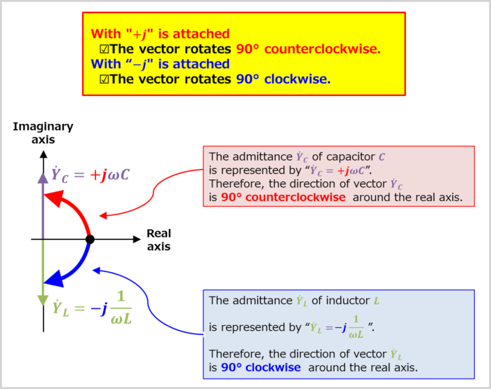
Here is a more detailed explanation of how vector orientation is determined.

The admittance \({\dot{Y}_C}\) of the capacitor \(C\) is expressed by the following equation

\begin{eqnarray}
{\dot{Y}_C}=j{\omega}C\tag{24}
\end{eqnarray}

Since the expression for the admittance \({\dot{Y}_C}\) of the capacitor \(C\) has '\(+j\)', the direction of the vector \({\dot{Y}_C}\) is 90° counterclockwise rotation around the real axis.

The admittance \({\dot{Y}_L}\) of the inductor \(L\) is expressed by the following equation

\begin{eqnarray}
{\dot{Y}_L}=-j\frac{1}{{\omega}L}\tag{25}
\end{eqnarray}

Since the expression for the admittance \({\dot{Y}_L}\) of the inductor \(L\) has '\(-j\)', the direction of the vector \({\dot{Y}_L}\) is 90° clockwise rotation around the real axis.

Admittance phase angle of the RLC parallel circuit

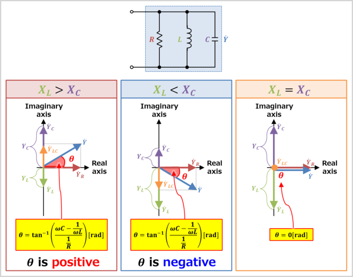
The admittance phase angle \({\theta}\) of the RLC parallel circuit can be obtained from the vector diagram.

\begin{eqnarray}
{\tan}{\theta}&=&\displaystyle\frac{{\omega}C-\displaystyle\frac{1}{{\omega}L}}{\displaystyle\frac{1}{R}}\\
\\
&=&\displaystyle\frac{\displaystyle\frac{1}{X_C}-\displaystyle\frac{1}{X_L}}{\displaystyle\frac{1}{R}}\\
\\
{\Leftrightarrow}{\theta}&=&{\tan}^{-1}\left(\displaystyle\frac{{\omega}C-\displaystyle\frac{1}{{\omega}L}}{\displaystyle\frac{1}{R}}\right)\\
\\
\\&=&{\tan}^{-1}\left(\displaystyle\frac{\displaystyle\frac{1}{X_C}-\displaystyle\frac{1}{X_L}}{\displaystyle\frac{1}{R}}\right)\tag{26}
\end{eqnarray}

From the above, the admittance phase angle \({\theta}\) of the RLC parallel circuit is expressed by the following equation.

The magnitude of the inductive reactance \(X_L(={\omega}L)\) and capacitive reactance \(X_C\left(=\displaystyle\frac{1}{{\omega}C}\right)\) determine whether the admittance phase angle \({\theta}\) of the RLC parallel circuit is positive or negative.

• In Case \(X_L{\;}{\gt}{\;}X_C\)
• In Case \(X_L{\;}{\lt}{\;}X_C\)
• In Case \(X_L=X_C\)

In Case \(X_L{\;}{\gt}{\;}X_C\)

If "inductive reactance \(X_L\)" is larger than "capacitive reactance \(X_C\)", the following equation holds.

\begin{eqnarray}
&&X_L{\;}{\gt}{\;}X_C\\
\\
{\Leftrightarrow}&&\frac{1}{X_C}-\frac{1}{X_L}{\;}{\gt}{\;}0\tag{28}
\end{eqnarray}

Therefore, the admittance phase angle \({\theta}\) of the RLC parallel circuit is "positive".

In Case \(X_L{\;}{\lt}{\;}X_C\)

If "inductive reactance \(X_L\)" is smaller than "capacitive reactance \(X_C\)", the following equation holds.

\begin{eqnarray}
&&X_L{\;}{\lt}{\;}X_C\\
\\
{\Leftrightarrow}&&\frac{1}{X_C}-\frac{1}{X_L}{\;}{\lt}{\;}0\tag{29}
\end{eqnarray}

Therefore, the admittance phase angle \({\theta}\) of the RLC parallel circuit is "negative".

In Case \(X_L=X_C\)

If "inductive reactance \(X_L\)" is equal to "capacitive reactance \(X_C\)", the following equation holds.

\begin{eqnarray}
&&X_L=X_C\\
\\
{\Leftrightarrow}&&\frac{1}{X_C}-\frac{1}{X_L}=0\tag{30}
\end{eqnarray}

Therefore, the admittance phase angle \({\theta}\) of the RLC parallel circuit is "\({\theta}=0{\mathrm{[rad]}}\)".

Summary

In this article, the following information on "RLC parallel circuit was explained.

1. Equation, magnitude, vector diagram, and admittance phase angle of RLC parallel circuit admittance

Thank you for reading.